Mineral Inversion at Scale

Mineral solvers, or mineral inversion models, have long-lived in the realm of the petrophysicist even though they provide superior results, especially in mixed lithology systems, compared to traditional methods where a single matrix density value is used for a zone. This has been driven by the perception that the models are a “black box” solution, beyond the comprehension of most geologists, and require specialist software and knowledge.

Historically, these models have often been slow… and in many software packages they are, with calculations times of 30 – 60 seconds per well. Although this doesn’t seem like much, when scaled to a project with 500 wells, this means you’ll lose a day in processing. 5000 wells? Forget it.

Danomics is changing the game and bringing these models to everyone working in the subsurface. We’ve focused on making them accessible to geologists with a straightforward interface and a large range of default minerals. We’ve also made them fast. Read on below to find out more.

What is a mineral inversion?

Mineral inversions, simply put, are just a method to determine the volumes of each mineral and fluid phase present in a rock. This is important because if we know the mineral composition and proportions, and the density of each of those minerals, we can calculate a grain density for the rock at each depth step – and this allows us to calculate a more accurate porosity.

This is especially relevant when you have mixed lithology or complex lithology systems like an organic shale where the kerogen volumes, associated pyrite, and non-shale minerals can vary substantially within an interval and across a play. Understanding these changes will allow you to more accurately calculate porosity, saturation, and geomechanical properties, and is therefore crucial to understanding the expected production and economics from drilling campaigns.

How inversions work

Mineral inversion modules are based on the principle that you can take the properties from a group of minerals (C) and multiply them by their relative volumes (V) to calculate the log properties (L). This is expressed in matrix form as:

C*V = L

However, in most cases we don’t know the proportion of minerals, but we do know the majority of minerals likely present and the log values. Therefore, we can invert the matrix to solve for their proportions. We thus rearrange as:

V = C'*L

where C’ is the inverse of matrix C. This simple matrix algebra then allows us to solve for the volume of each mineral (V). In Danomics’ Inversion module we seek to minimize the error between the predicted logs and the actual logs, weighting by the confidence we have in that log measurement. Danomics’ inversion simultaneously forces the constraint that all mineral proportions honor the requirement that 0 <= V <= 1. That is, you can’t have mineral volumes that are negative or greater than 100% (this is mathematically possible, but not physically possible).

When shown in this form, it shows you that an inversion is basically just some matrix algebra at its core. It gets a bit more complex in that we typically don’t list out every single mineral that is possible and we also don’t have perfect log responses. That is why we need to use an iterative “solver” that will find the best match for us (this will be important later when we talk about speed). As an interpreter, what you really need to know is the following:

• The minerals that make up the majority of the rock.
• The mineral properties..
• That the system will generate “predicted” curves and that those curves should be as close as possible to the input curves.

With respect to the minerals that make up the rock you can either use knowledge of the depositional system, core data, or cuttings data to inform your mineral selection. You composition will often be something like quartz, feldspar, calcite, and shale for a sandy systems or calcite, dolomite, siderite, and shale for a carbonate system. For an organic shale you’ll want to include kerogen and pyrite as well as your more typical matrix minerals like shale, calcite, and quartz.

The mineral properties you’ll need are available in vendor chartbooks, text books, and publications. These are usually easy to find and for our pre-determined mineral list Danomics has a list of the properties you’ll need as defaults.

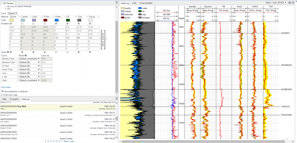
In the figure at the top of this section we show a screenshot of a log panel with actual curves (black), predicted curves (red), and the error bands we want to stay within (yellow). The objective here is to get the best overall match possible and to have all of the curves within the yellow bands.

You may be wondering, how exactly do you “predict” curve values. This is easier than it sounds and can be demonstrated with a quick example. Let’s imagine we have a rock that has 60% quartz, 20% calcite, 10% dolomite, and 10% porosity that is filled with water. If we wanted to predict a density curve we would say:

RhoB_Predicted = 0.60*2.65 + 0.20*2.71 + 0.10*2.87+ 0.1*1

The values above represent the volume of quartz * density of quartz + volume of calcite * density of calcite and so on. This means that the predicted density is 2.52 g/cc. (to calculate the grain density we leave out the porosity and divide by the sum of the remaining minerals – in this case it is ~2.69 g/cc). The same procedure can be done for neutron, sonic, PE, or any other curve.

Now that we have demystified the math, let’s take a look at the mechanics of doing the inversion before we head on to how Danomics has made this lightning fast.

Setting inversion parameters

There are several available parameters in the inversion module, and care needs to be taken when setting each. This section will review each parameter and how it is best used.

The Zone parameter determines which zones the rest of the parameters are applied to. If you only enter parameters for the default they will be applied to each zone in the same way. However, you can fully customize each zone individually, or only certain zones. Best practice typically goes as follows:

1. Set the mineral composition, properties, and curves for the “Default”
2. Navigate to different zones of interest and customize the parameters for that zone(s).
3. If subsequent changes are made to the default, check zones with customizations to ensure that they still have the desired parameter values.

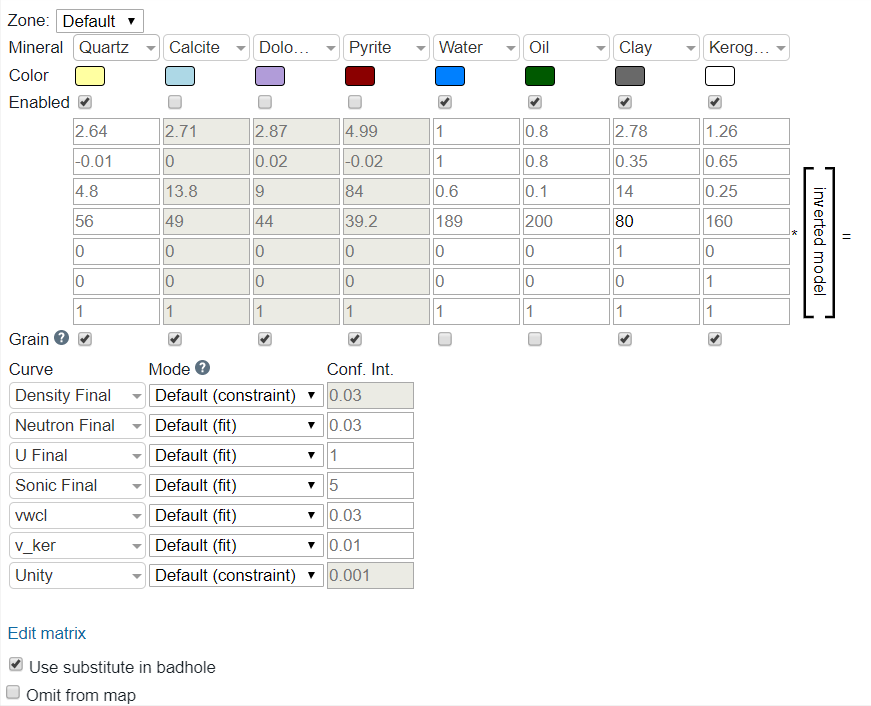
The Mineralparameter contains a list of ~15 options that can be selected. These correspond to the components (C) that we will be solving the proportions for during the inversion. The default composition is for Quartz, Calcite, Dolomite, Pyrite, Water, Oil, Clay, and Kerogen. However, this can be changed by selecting the desired minerals for the Default or on a zone by zone matrix. Additional minerals can be added by clicking the Edit Matrix link at the bottom of the table. This link also allows for changing the order of the minerals as well.

When a mineral is selected, its default properties are present by default. These values are reference numbers from various vendor chartbooks and academic papers, and are fully editable by the user. Additional minerals can be added via editing the CPI Config (advanced users only; please contact Danomics’ help staff if you need to edit the list of available minerals).

There are two special cases in Danomics’ mineral list – these are Clay and Kerogen. Clay corresponds to the final Vclay (vwcl) calculated in the Vclay module. Kerogen corresponds to the volume of kerogen (v_ker) calculated in the TOC module (technically a conversion from TOC wt. % that is done automatically for you). Danomics adopted this workflow from the work presented by Newsham et al., 2019 in the SPWLA 3 part tutorial on evaluating organic mudstones.

The Enabled parameter simply allows one to turn minerals on/off. When turned off the mineral is omitted from the inversion and the properties are grayed out.

The Properties Matrix as shown below corresponds to the mineral properties for each log curve:

In the default configuration this corresponds to RhoB (density_final), Nphi (neutron_final), U (u_final), DT (sonic_final), Vclay (vwcl), Vker (v_ker), and Unity. For clarity, below is the list with an explanation of each:

• RhoB: Bulk density of each mineral (e.g., calcite has a bulk density of 2.71 g/cc).
• Nphi: Neutron value of each mineral (e.g., calcite has a Nphi value of 0.00).
• U: U is the product of the bulk density and photoelectric curves such that U = PE*RhoB. This needs to be tuned, especially for Clay.
• DT: The compressional sonic travel time in uSec/ft for each mineral (e.g., calcite has a DTc of 49 uSec/ft).
• Vclay: The proportion of each mineral that is clay. This is zero in all cases, except for Clay, in which the value is one. This essentially tells the inversion that the Vclay from inversion should equal the Vclay from the clay volume module.
• Vkerogen: The proportion of each mineral that is kerogen. This is zero in all cases, except for kerogen, which is a value of one. This essentially tells the inversion that the Vkerogen from inversion should equal the Vkerogen from the TOC analysis module.
• Unity: This dictates that the mineral composition should sum to a value of one.

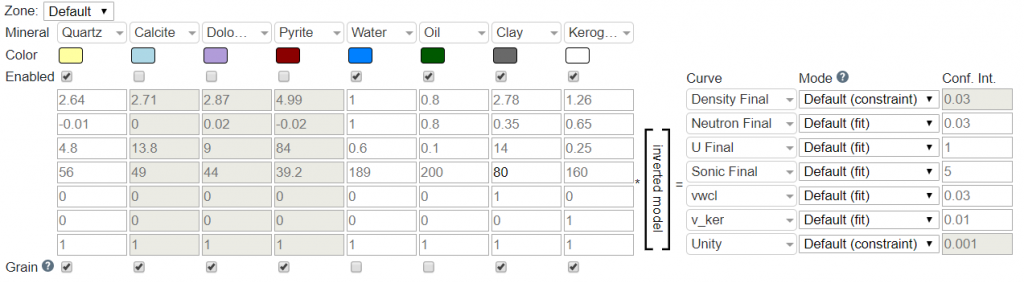
The Curve parameter dictates which curve the properties correspond to in the inversion. E.g., if you have the first row as the mineral property for bulk density, the first curve should be the bulk density curve (density_final).

The Mode parameter instructs the solver on how to treat the curve. Options are “Fit”, “Constraint”, and “Disabled”. These are defined as follows:

• Fit: The solver will try to minimize the difference between the predicted curve from our inversion and the actual log curves, with each weighted by its confidence.
• Constraint: The solver will treat the curve as a constraint, and will force an exact solution.
• Disabled: The solver will ignore the curve in the inversion.

Danomics’ uses constraint as the default for RhoB and Unity, with fit as the default for the remainder of the log curves. Constraint as used as a default for RhoB and Unity because if those curves are forced to an exact solution then the density porosity from the inversion will exactly match the density porosity from the density porosity equation. However, this is not a requirement and they can be set as fit as well. This will result in some deviation between the density porosity equation and the porosity volumes from the inversion (where porosity volume is the sum of oil + gas + water).

The Conf. Int parameter is the confidence in the curve value that is used in establishing a fit (i.e., the weighting). Lower values equate to higher confidence. In the screenshot above, the U Final has a lower Conf. Int. than the Sonic Final curve. This does not mean that the curve is more accurate or of higher confidence… one must keep in mind that the curves have different ranges with U Final typically <15 while Sonic Final can range from 40-200 depending on the constituent. The default values are sourced from various academic studies, but there is no definitive value for any given curve, especially when working with large data sets that cover different vendors and tool generations. The general rule of thumb is that the confidence should be somewhat proportional to the range of variation observed in the data.

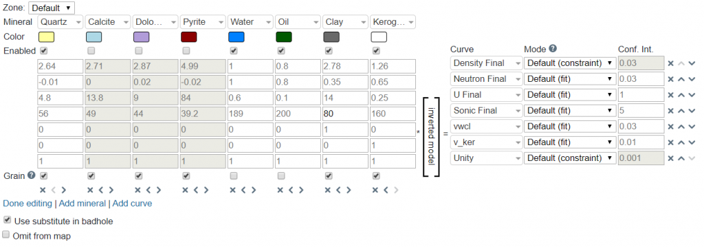
When Edit Matrix is clicked, it will bring up controls that will allow one to configure the matrix layout. Options are to shift minerals left/right, shift curves up/down, add minerals, add curves, and delete minerals/curves. The matrix can be reset to the default if undesired changes are made. When finished, simply click on Done editing.

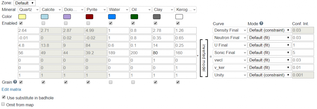
The Grain parameter should be checked for components that will be used in determining grain density. For example, quartz, calcite and dolomite are all “grains” while oil, water, and gas are not “grains”. So, if it is a mineral/rock then select “grain”, and if it fills a pore space turn off “grain”.

The final parameter specific to the mineral inversion module is the Use substitute in badhole. If selected this will utilize the synthetic RhoB derived from the parameters in the Bad hole ID & Repair module calculated via the Gardener relation (i.e., from the sonic curve).

Making inversions fast

Earlier you’ll recall that I mentioned that we use a “solver” to get the composition. This is how all modern petrophysics software packages perform inversions. However, not all solvers are created equal and not all approaches are created equal.

In general, solving for a system of equations isn’t that difficult – you try to find a value to minimize on and then you start varying parameters until you converge on a solution. This process gets complicated when you start adding constraints (such as no negative values or no values greater than 100%). With some packages you might run 30-50 iterations before converging on a final solution.

This process can be handled by a number of “off the shelf solutions”, and if you’re running it on a single well, like most petrophysical packages its okay if it takes 30 seconds or a minute to run. However, if you are running it on large projects with 1000s of wells that is unacceptably slow. That is why Danomics chose to use a more custom solution that allows us to typically solve the system of equations required in < 1 second (typically less than 0.1 seconds). And this is what has allowed us to start performing inversions at the basin scale.

And, perhaps a bit unsurprisingly, mineral inversion models are often extremely reliable over large areas. The reason for this is easy – although mineral proportions can change substantially as we move across the depositional system, the mineral mix doesn’t. For example as you move from a shoreface sand to the shallow marine and into the deeper marine environments your mineral composition is often the same, its just the mix of sand and shale that is changing as you move outboard in a system.

Parting thoughts

As the industry has moved from capturing acreage into more intensive development with substantial capital outlays in a difficult price scenario, it is more important than ever that we drill the best wells on the best acreage… and this means moving beyond both cutoff mapping and simple log analysis and moving toward using robust petrophysical workflows for our daily mapping work.

Part of that transition is to move toward using more accurate methods like mineral inversions to determine grain density (and hence porosity). This may require re-tooling with respect to which software packages get used, but in the end a bit of effort spent learning a new tool combined with the low costs of cloud-based solutions is far less than the cost of drilling sub-optimal wells.