There are instances when you may not want to use either a fixed value or a dynamically re-mapped value for a petrophysical parameter. For example, in your TOC calculation you may wish to have the maturity (Vre) vary spatially from well to well, or for a property like the gas-oil-ratio that is used in the volumetrics calculation you will rarely use the same value across a play and will want to vary it based on known production data. For these types of use cases Danomics has developed the concept of “interpolated parameters”. Interpolated parameters will allow you to:
- Import or create a table of values for a petrophysical property
- Grid that table of values using Delaunay triangulation
- Assign the values from the grid to other wells.
This is show schematically in a simple example below:
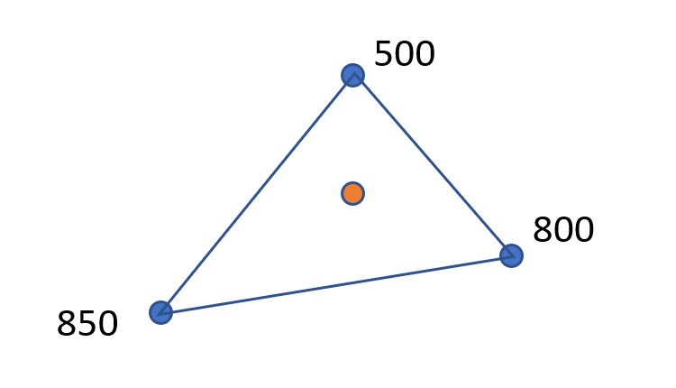
In this example there are three known values for a parameter (blue points) and a well with an unknown value (orange point). Using a triangulation between the three points we can calculate a value for the orange point of about 715. This value is based off a grid made between the three wells with the known values. For properties that follow trends (such as gas-oil ratio or maturity) this is a powerful tool. It means that we can interpret/input the values from a small number of wells, and then use those values to determine the values for a large number of wells.
Creating/uploading a spatial table
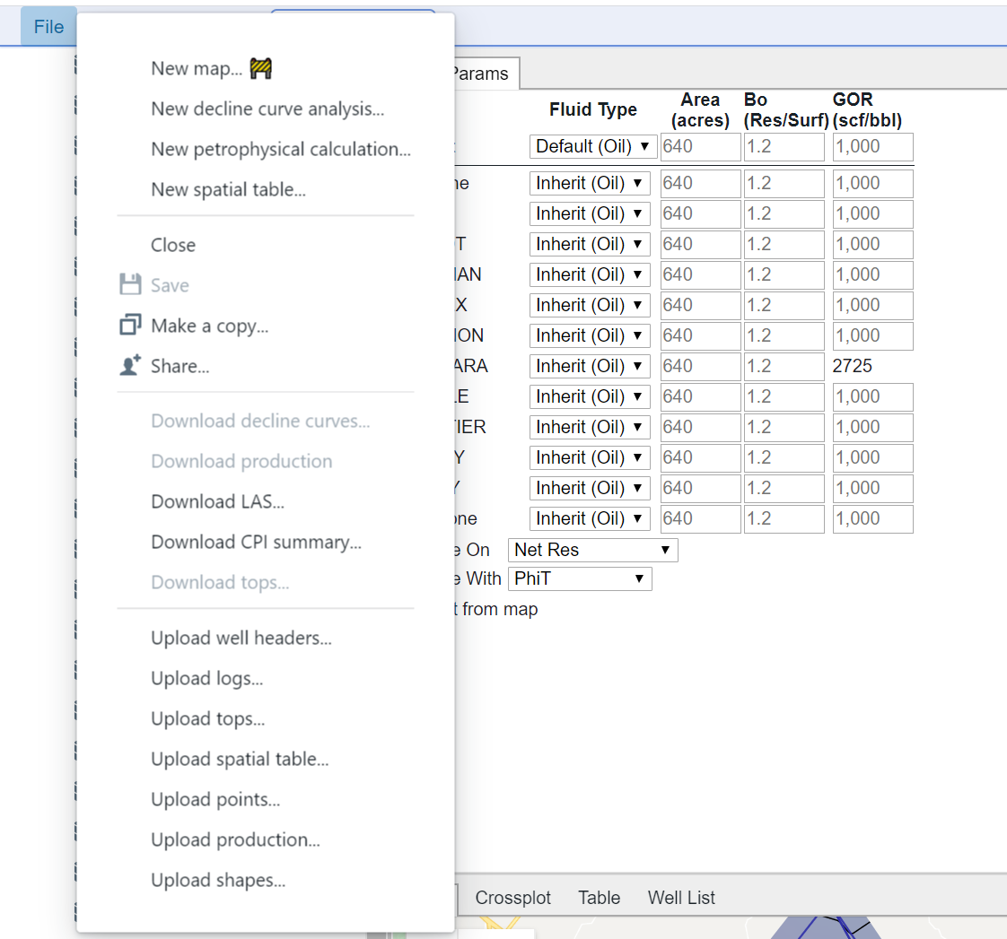
To create a spatial table there are two options:
- File >> New spatial table…
- File >> Upload spatial table…
This dialog is shown here:
If you select “New spatial table” you will be presented with the following dialog:
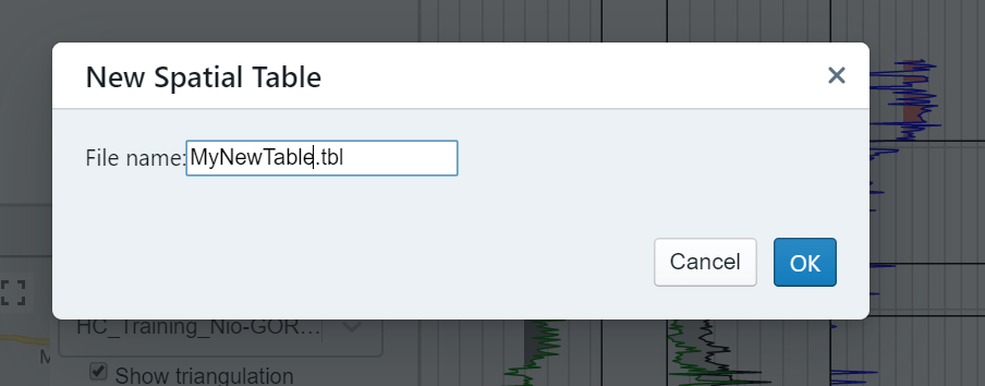
Simply provide a name and click okay and you will have created a new blank table. This table can then be populated by making entries in the wells as individual interpretations for that property are made.
If “Upload spatial table…” is selected you will be taken to the following dialog:
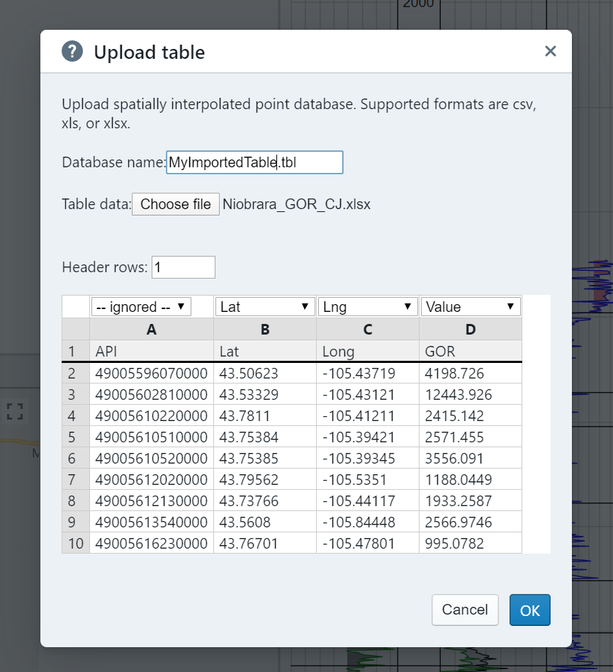
In this dialog you will select your file and then you will need to assign the following mandatory columns:
- Lat: The latitude of the data point
- Long: The longitude of the data point
- Value: The value of the data point
In the example above for reference the API column was left in the spreadsheet, but it is ignored by the importer as it is not used in the triangulation process. For the value above we are importing GOR (gas-oil ratio). You can use any name that you desire. If duplicate lat/long coordinates are included on the first value will be kept.
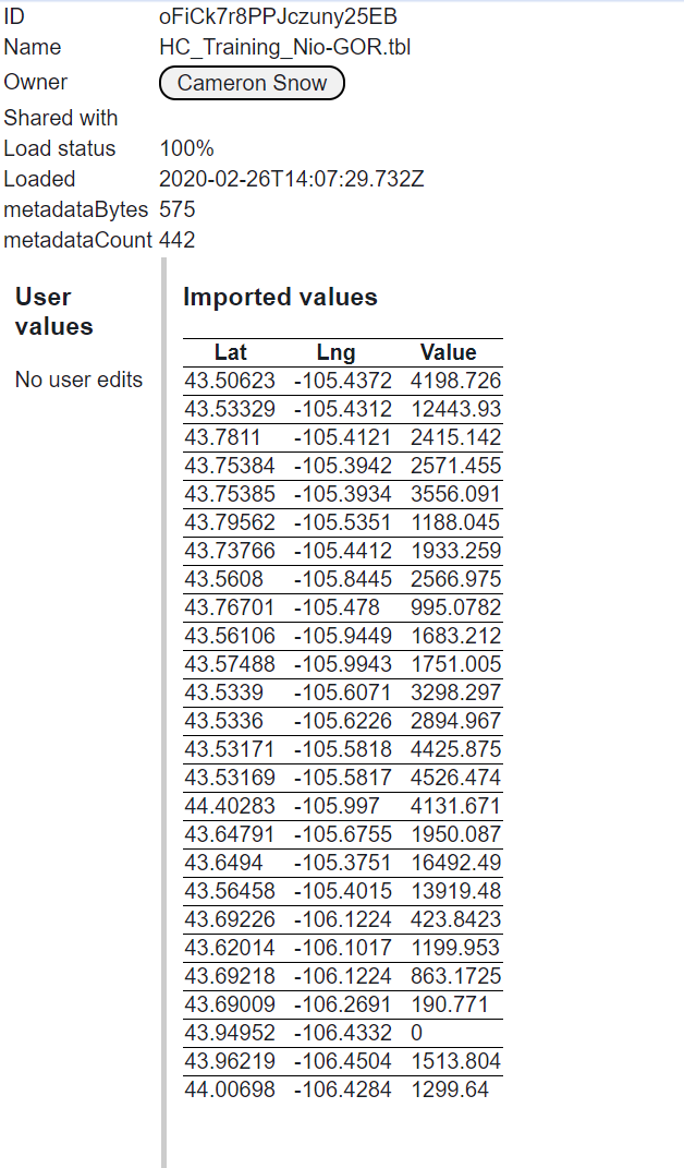
Once the import is complete you will see the imported values as below:
Using the spatial table
When you hover over a cell in a parameter table you will be shown a “setting icon”. If you click on the icon the following dialog will appear:
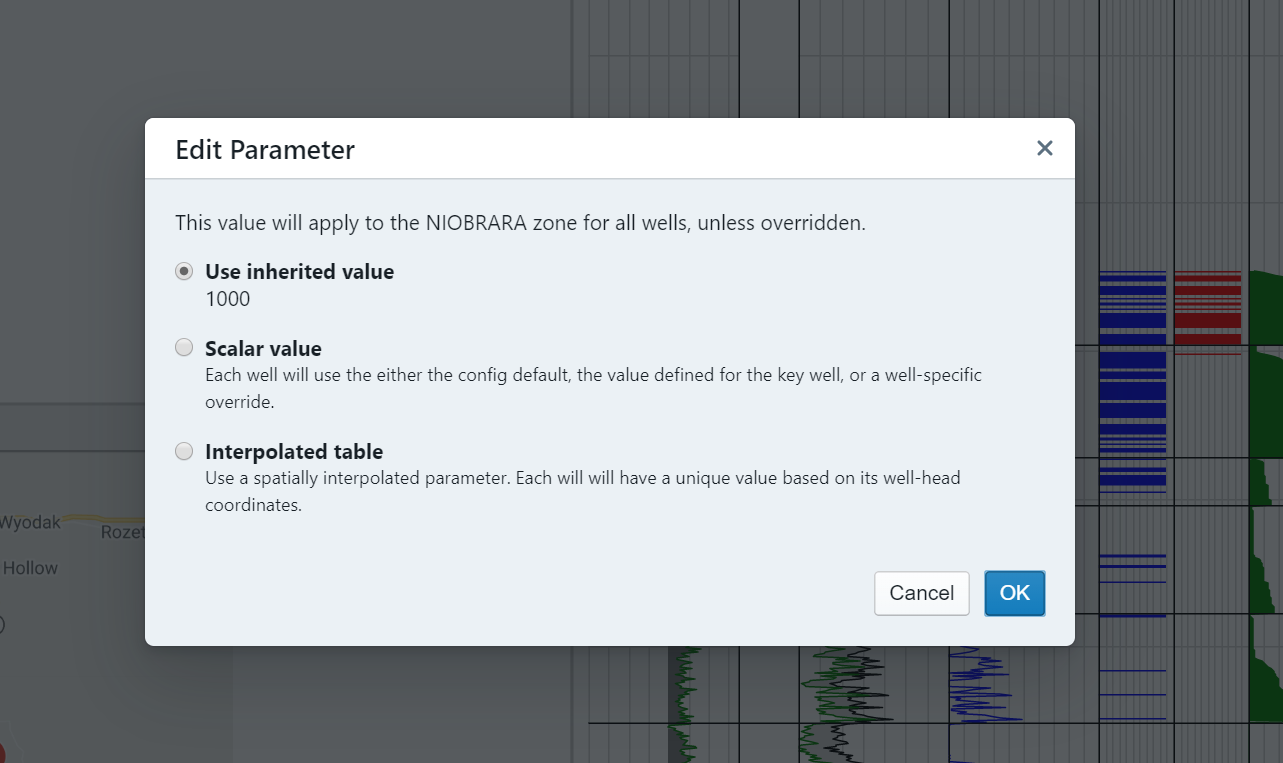
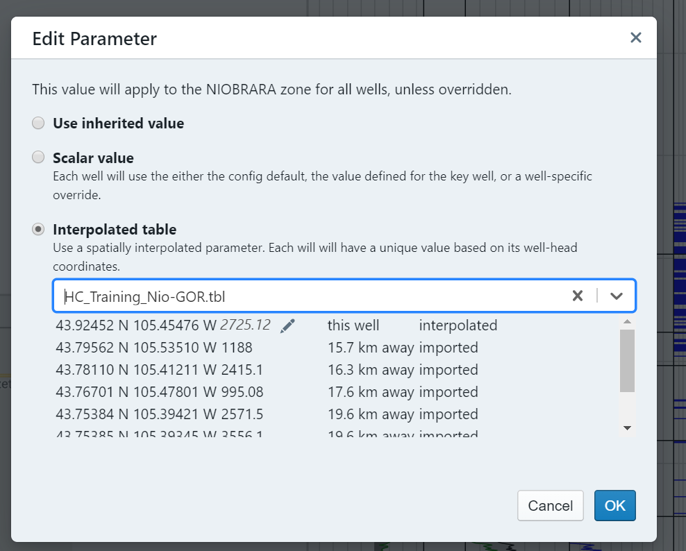
This table gives you the option to use the inherited value, a scalar value, or an interpolated table. If you select “Interpolated table” you will then be able to choose the desired table and will see a preview of the data points:
Once you click okay, the table will be applied to the well.
Note, you should always have the spatial table applied to the key well! Not doing so will result in unexpected results.
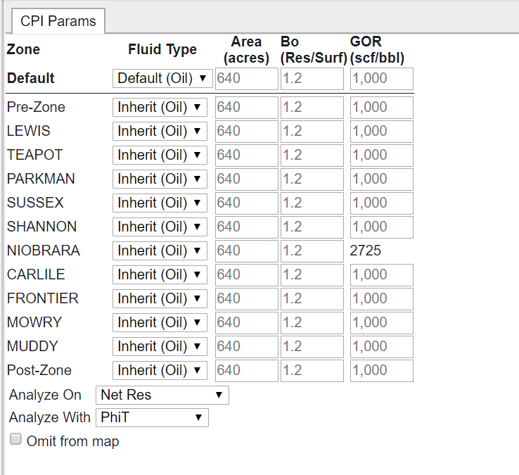
Once you have applied a table to a parameter, you can verify this visually by noticing that the parameter entry box will now disappear and there will simply be a value present.
Adding data to a spatial table
To add data, click on the settings icon beside the value. Doing so will bring up the following dialog:
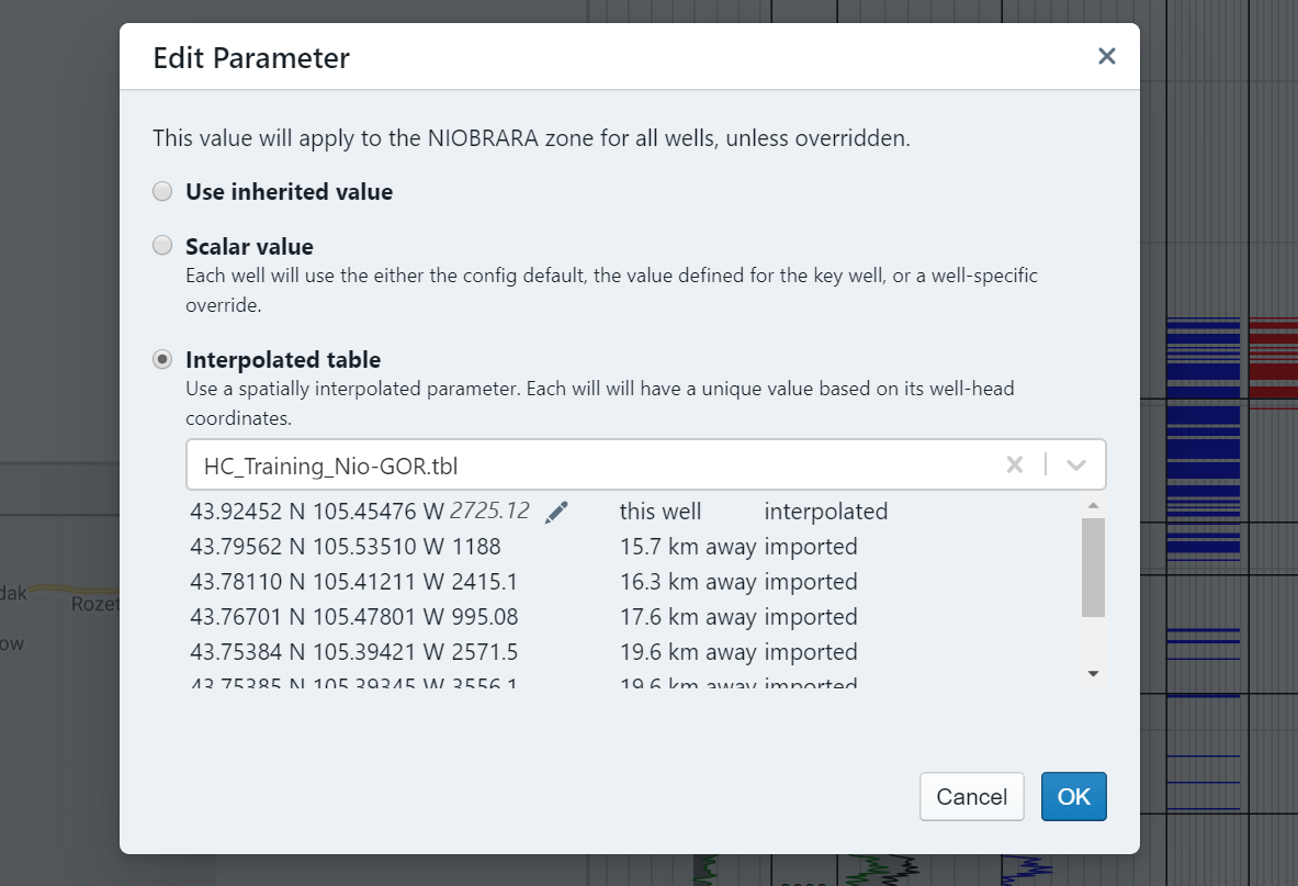
You can see in this example, there is no value for the well we are on. To add a value to this well, click on the pencil icon and an entry box will appear. Enter the value, click outside the box, and then click OK to apply. You can verify that the value has been entered by clicking on the table and looking at the preview:
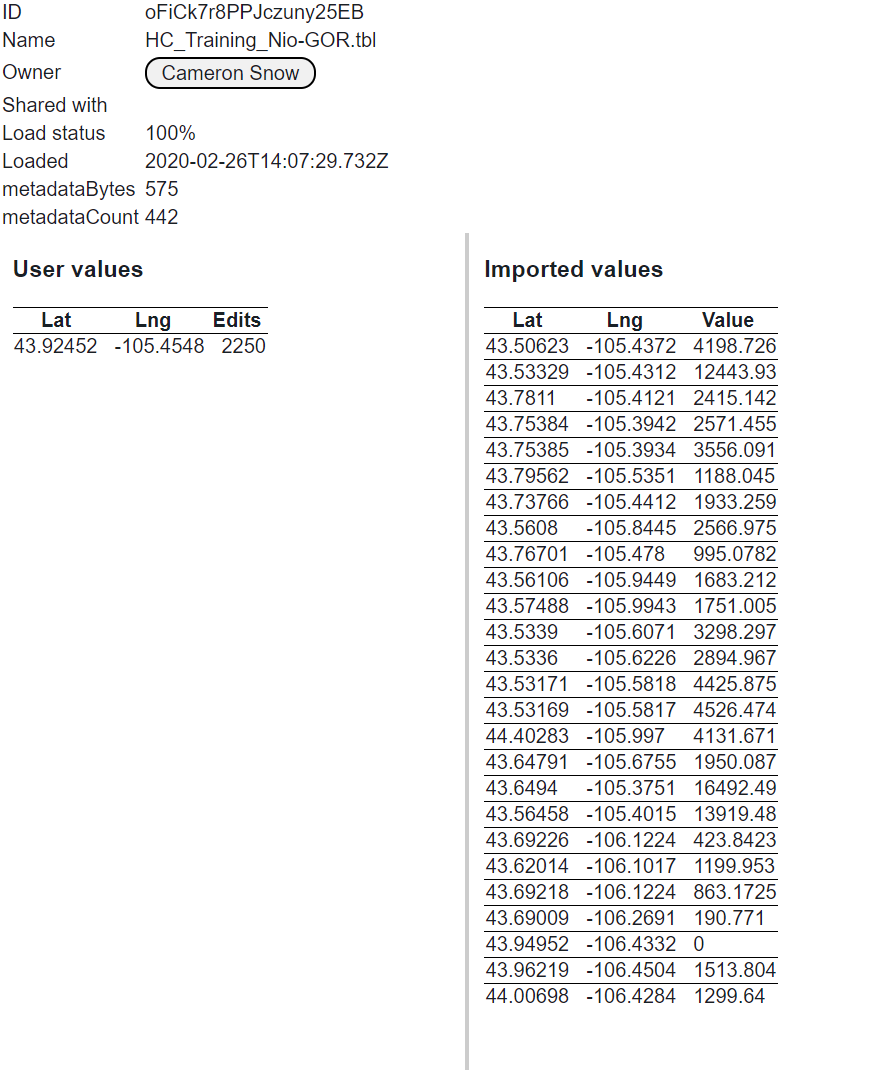
The “User values” will show all of the values that have been manually added to the table.
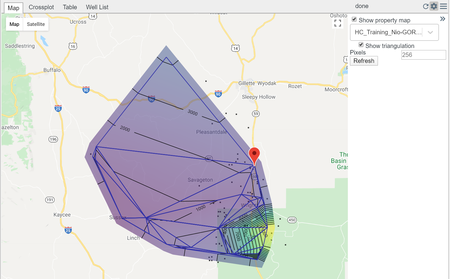
Mapping the table
To better understand where the petrophysical parameter values are coming from there is an option to both map the table values and display the triangulation lines. This is done via the normal mapping tab, as shown below:
Tips and tricks
- If using a spatial table make sure that it is applied to the key well. Not having it on the key well will likely result in unexpected behavior.
- If you want to remove the spatial table, click on the setting icon on the key well, and enter in a “scalar value”. This will take it back to the “normal” state.
- Try to create a regularly spaced grid of data points
- Stay tuned to this page – more updates are coming!