Removing Outliers from Maps

One issue that is common when generating maps and grids is that there will often be a few outliers – this is especially true when working with large, disparate data sets. There are several ways to approach outlier removal, including:

• Removing wells from the data base
• Smoothing away minor anomalies
• Filtering gridded values based on spatial statistics

Removing wells from the database, although the most straightforward, is using a blunt instrument to address the problem. This will affect all zones and all properties. Smoothing away anomalies can sometimes work, but more often than not a filter effective enough to remove a large bulls-eye on a map will remove other important trends. That is why in this article we will review how to use spatial statistics to remove outliers on a zone-by-zone, property by property basis. We will do this using Danomics Flows tools.

Making a Grid in Flows

The first step in this process is understanding how to make a grid using a standard Flow. To do this we’ll add the following blocks:

1. Log Input
2. CPI Log Calc
3. Points Select
4. Points To Grid
5. Grid Output

Here is what the completed flow will look like:

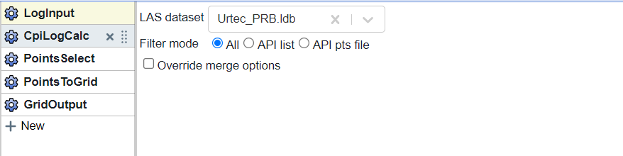
In the LogInput block you should select the log database that you want to create properties for. If you only want to use a subset, choose to filter using either an API list or points file.

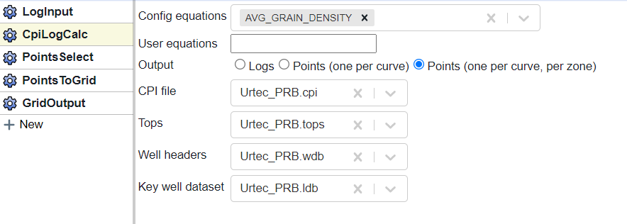
In the CpiLogCalc block (shown above) you will want to select a property (or multiple properties). Since we are going to generate a grid for a specific zone, we’ll set the output to “Points (one per curve, per zone)”. Since we are generating output from a file we have already interpreted we will select the CPI file, Tops, and Well headers of interest. If a key well was used in the interpretation you will need to select the log database that has the key well (usually the same as the one in the LogInput block).

This will output points for each zone and each selected property. Since we only grid one zone at a time, we need to use a PointsSelect block to select the values specific to one zone.

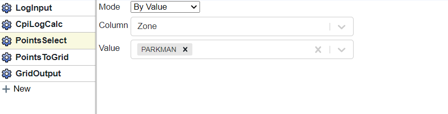
Here, in the “value” dropdown menu you should be presented with a list of the zones available. In this case, we are making a map on the Parkman formation.

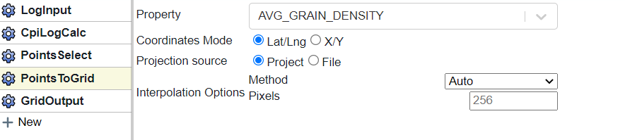
In the PointsToGrid block we select the property to grid. We can also set the options for coordinates and and gridding options here as well.

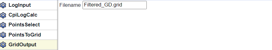
Finally, we use the GridOutput block to assign a name to the grid file we are writing.

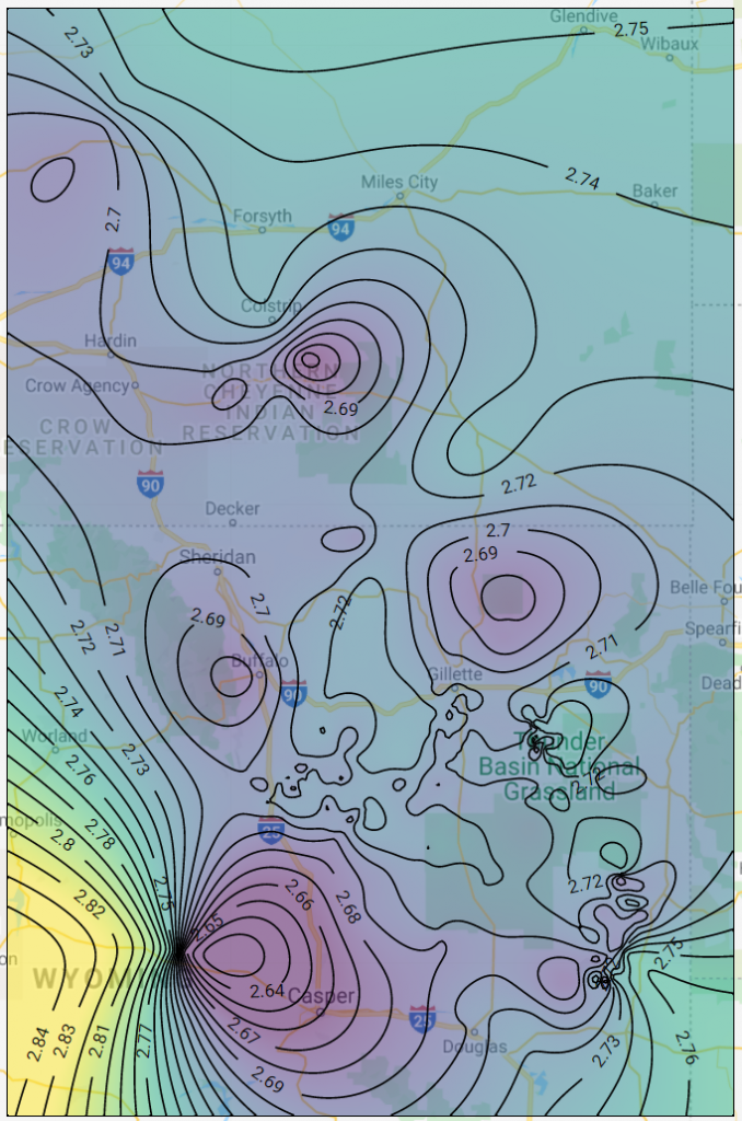
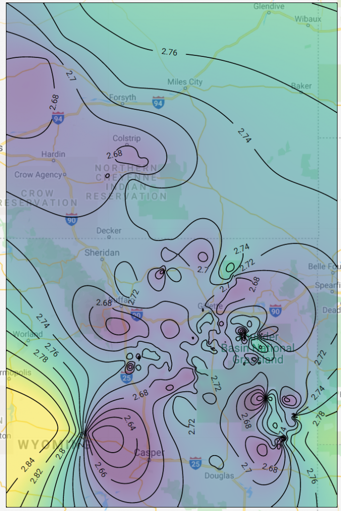
We then run the flow by clicking the “play” button. Here is the result from the flow I just built.

Applying Spatial Filtering

Now that we have made a grid, it’s now time to apply spatial filtering to apply clean-up. Danomics using spatial-based filtering because if working in large areas there are often natural variations that make using absolute values untenable. Therefore, we look at the statistics from a specified number of offset wells and evaluate if a well falls outside an acceptable range.

The way this works is that it looks at specified percentiles for n-offset wells (p10 and p90 by default), then takes the difference between those values and multiplies it by an outlier ratio. So if the P10 is 30, the p90 is 50 and the outlier ratio 0.5 it will filter values less than 20 and greater than 60. This is arrived at by (50-30)*0.5 = 10, and 30-10 = 20 and 50+10 = 60.

To apply this block we will add it to the Flow we made above, so that:

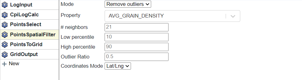
In this example we set the property as the one we wish to grid, define the number of neighbors, the low/high percentiles, and the outlier ratio. The closer together the percentiles and lower the outlier ratio, the more aggressive the filter would be. For example setting the Low/High percentiles at 20/80 with an outlier ratio of zero would essentially remove any value that falls outside of the p20/80 range. It’s worth experimenting with to get a feel for your specific data.

Here is the same map as above, but with the filtering applied.