Within flows the CpiLogCalc block allows you to take advantage of your petrophysical interpretation as well as the petrophysics infrastructure including the equations and functions. This article reviews how to use the native Config equations as well as User equations.
Prerequisites
Before you start with a CpiLogCalc block you will need to provide the input to it. This will require that you have a LogInput block beforehand. You should add that component and select the relevant log database.
To take full advantage of the CpiLogCalc‘s capabilities you should have already performed your petrophysical interpretation. Although this is not required, it will provide you with substantially more options and will allow your customized interpretation to be used in the Flows tools.
CPI, Tops, and Well headers selection
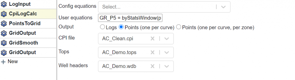
There are three dropdown menus:
- CPI file
- Tops
- Well headers
The CPI file option is what allows you to bring in your petrophysical interpretation. This will allow you to have your key well, parameters, and other customizations available to the Flow for further use.
The Tops option allows you to bring in the relevant Tops Database. This is required if you want to perform operations that should operate on a zone-by-zone basis. This should be a tops file that is relevant to the selected CPI file.
The Well headers option allows your project to be spatially aware. This is important if you want to perform further gridding operations. It should be a well headers file that is relevant to the selected CPI file.
Output Type
You can choose to output either Logs, Points (one per curve), or Points (one per curve, per zone). Your selection will depend on what you wish to do next. A brief explanation is given below:
- Logs: If you plan to subsequently perform an operation on, or to export, the log database you should select this option.
- Points (one per curve): This option is if you wish to calculate a single point for the well for a curve. This is the option should typically be used in conjunction with a user equation that is wrapped in “byStatsWindow” (more detail below).
- Points (one per curve, per zone): This is the option to use when you wish to generate points on a per zone basis. For example, if you wanted to make a map of average porosity by zone, this is the option you would use.
Config Equations
This tool allows you to have access to all of the default equations available in a CPI Config file. This means you can access the most relevant curve names (see reference here). In the example below I have selected the equations for total and effective porosity (phit and phie).
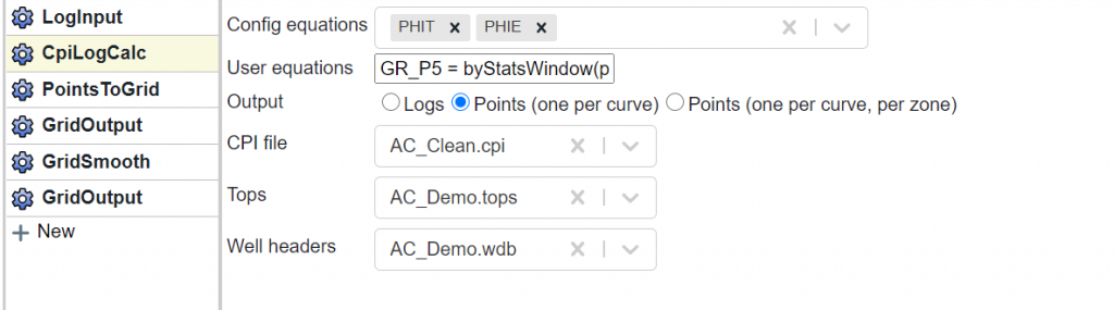
In this example, since I have selected a CPI file, this means the PhiT and PhiE curves will be calculated using the parameters that I interpreted in the “AC_Clean.cpi” file.
User Equations
User equations are what unlocks the ability to make true customizations to your exports. However, this does require that you understand how operate in some detail.
Most calculations in Danomics operate on a depth-step by depth-step basis. For example, if you think about the porosity equation a calculation is performed at each depth step independent of all other depth step. However, if you wish to average the porosity by zone or generate a cumulative PhiH curve, this uses information from multiple depth steps.
When generating curves we typically operate sample by sample, while when generating points for mapping we generally operate on multiple samples.
When operating on multiple samples we need to wrap equations in either a “byFormation” or “byStatsWindow” function. For example, if we wanted to evaluate the 5th percentile of the gamma ray curve for each petrophysical zone in our analysis we would use the following:
GR_P5 = byFormation(percentile(5, @gr_final))The above will calculate the 5th percentile of the gamma ray final curve on a zone by zone basis. However, if we want to calculate it over our entire statistics window (as defined in our CPI file) we should use the “byStatsWindow” function as shown here:
GR_P5 = byStatsWindow(percentile(5, @gr_final))Note that you will have access to all of the pre-configured summary curves. This includes many of the averages and summations that are likely relevant to your analysis (all of which are shown in the map dropdown list in your CPI file).
Tips and Tricks
- Remember you can find most of the relevant curve names in this reference guide.
- You can also go to the settings (head icon in top right corner) and open the CPI Config. In this file you will find all of the available equations for each module. The “Export.yaml” file contains all of the summary curves for an analysis.
- To determine the output type (Points vs. Logs) think about what your next operation will be. If it is making a map, points is typically the way to go.