In Danomics Petrophysics users are guided through a workflow that walks them through a number of modules. These modules are located via a dropdown menu at the top center of the window. The modules are listed in the order in which a user should ideally proceed through a project. However, this order is not strictly enforced and the user can start at any module and can seamlessly move both forward and back through the modules. This help article will focus on the Shear Wave Modelling module.
Shear Log Modelling
Use Cases
The Shear Log Modelling module is intended to help users generate a calibrated shear sonic log for wells in which only a compressional sonic log was measured, as is often the case. The module uses the Greenberg and Castagna methodologies for calculating a synthetic shear log that can then be used in other calculations, such as in the geomechanics module or the fluid substitution module. A common workflow may be to:
- Identify a well that has a shear sonic log
- Interpret that well through each module through the water saturation
- Navigate to the shear log modelling module
- Identify the parameters that create a good fit between the observed and modelled shear sonic (DTS) curves
- Apply that calibration by using those parameters in the key well (if the present well is not the key well)
- Use those curves in the geomechanics, fluid substitution or other modules.
Shear Log Modelling parameters
To access the Shear Log Modelling module use the dropdown selection menu located in the top-center area of the window and select the “Shear Log Modelling” option.
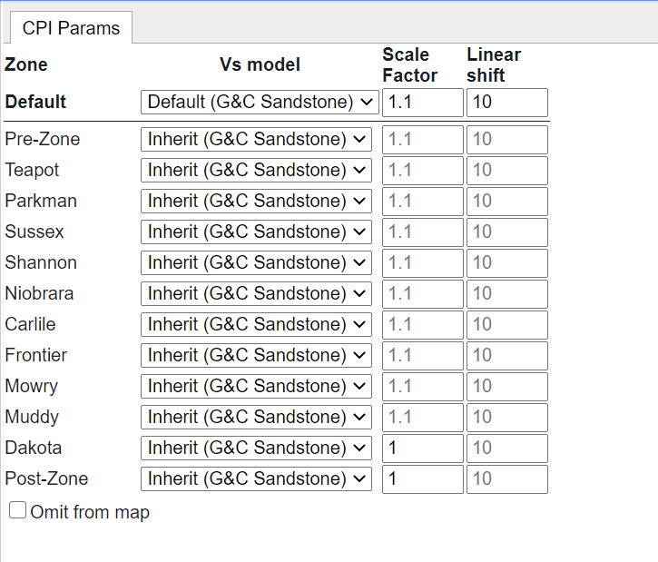
Once the module is active there are three parameters that can be set on a zone-by-zone basis. These are the Vs Model to be applied, a scaling factor and a shifting factor.
The Vs Model option allows you to select the model that best fits these observed data. Options include:
- Greenberg & Castagna Sandstone
- Greenberg & Castagna Limestone
- Greenberg & Castagna Dolomite
- Greenberg & Castagna Shale
- Blended Lithology model
- Mudrock Line model.
The Greenberg & Castagna models use the given end-member lithology to reconstruct the shear wave, while the blended lithology model uses the mineral proportions from the mineral inversion module in combination with published mineral properties to determine the shear log response. The Mudrock line model from Castagna et al. to calculate the shear log.
The Scale Factor parameter is a multiplier to help you stretch or squeeze results to obtain a better fit between the observed and calculated DTS curves. The Linear Shift parameter is a simple addition/subtraction from the calculated DTS curve, also designed to help obtain a better fit between observed and calculated results.
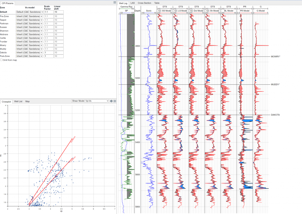
Calibrating and QC’ing the Model
The log tracks displayed show the results from each of the Greenberg & Castagna end-member models and the Blended Lithology model against the observed DTS log. Red shading indicates the observed DTS is greater than the calculated DTS, while blue shading indicates the opposite. In an ideal match there is very little difference between the curves. The user should evaluate each of the models on a zone-by-zone basis and select the model that gives the best fit in each zone, accounting for their understanding of the lithology. The scaling and shifting parameters can be subsequently applied, however, best practice is to keep the scaling factor as close to 1 as possible and the shifting factor as close to 0 as possible.
There are additional tracks for model QC. The observed vs. modelled Poisson’s ratio track can highlight areas of impossibility (e.g., PR > 0.5 or < 0) as well as highlight areas of severe misfit once the model has been set and calibrated for each zone. A second track shows the modelled and observed shear modulus (G). Once again, after all calibration has been finalized a substantial mismatch between these two would suggest that the model is likely not ideal.
Key Outputs
The following table provides a listing of some of the key curves used and generated in this module. Key outputs are given in bold font.
| Description | Mnemonic | |
| Input shear sonic log | dts_final | |
| Synthetic shear sonic log | dts_synthetic | |
| Final DTS log that is a composite of the input DTS, when available, and synthetic DTS when not available. | dts_rphys | |
| Greenberg & Castagna shear log model results (sandstone) | gc_ss_model | |
| Greenberg & Castagna shear log model results (limestone) | gc_ls_model | |
| Greenberg & Castagna shear log model results (dolomite) | gc_dol_model | |
| Greenberg & Castagna shear log model results (shale) | gc_sh_model | |
| Blended Lithology shear log model results | dan_vs_model | |
| Mudrock Line shear log model results | mudrock_model |
Troubleshooting
Remember that very few wells in your data set likely have a DTS curve, so it can be useful to use the Filters and set the required logs to “Custom” and enter “dts” in the search box. However, remember to remove this filter once you are ready to move along to other workflows that you want to apply to the broader set of wells.
For many of the results you need to have a porosity calculation available. Make sure that you have set the porosity model in the Porosity Interpretation module before starting the shear log modelling. Ideally you will have completed the Badhole ID & Repair, Clay Volume, TOC Analysis, Mineral Inversion, Porosity Interpretation, and Water Saturation modules before embarking on shear wave modelling as they will impact the results.
An ideal approach, if you have two wells with DTS curves, is to set the parameters on one, and use the other for a blind test. Although this can work at scale and across large numbers of wells, if you need precise results you will need to test your calibration across several wells to gain confidence that it is delivering the desired results.