Danomics provides beta access to some of our internal R&D tools before they are officially supported. This gives customers a way to access cutting edge technologies while we collect customer feedback. While in the R&D stage these tools are regularly enhanced and modified, and backwards compatibility is not always guaranteed.
Why use the Property Prediction tool?
It is unlikely that the results from this tool will provide a superior result to a manual analysis performed by a petrophysical expert with a deep understanding of the data and the geographical context of the well. However, there are several reasons to consider running the model. These include:
- Rapid results that require little to no user interactions
- Results can be used to guide interpretations, which can be especially useful for non-petrophysicists
- Results can be used as an “audit” of manual results – large variations between the manual and ML-based results can highlight areas that may need a more in-depth review
ML-Based Petrophysical Property Prediction
Danomics’ machine-learning based petrophysical property prediction tools were trained using a data set comprising over 1500 well logs from around the globe that were interpreted using Danomics proprietary interpretation methods. The data set comprises both conventional and unconventional reservoirs and a wide array of reservoir and non-reservoir lithologies. The interpretation process was a follows:
- Application of Danomics Interpretation Ready Data workflow to ensure data completeness, consistency, and quality
- A multi-well interpretation for clay volume, toc estimation, mineral inversion, porosity determination, and water saturation calculation
- A rigorous QC of results to ensure accuracy across the data set.
Benchmarks on petrophysical property prediction were then established using random forest and gradient boosting methodologies. In all cases the mean absolute error (MAE) was used as the metric for judging model efficacy as it was deemed to be more understandable than metrics such as mean squared error. Benchmark values for accuracy are as follows:
- Clay Volume: 4.3-4.7% MAE
- TOC Estimation: 0.3-0.4 wt% MAE
- Grain Density: 0.03-0.10 g/cc MAE
- Total Porosity: 1.5-2.0% MAE
- Water Saturation: 7.5-10.8% MAE
For clarity on the above benchmarks the values are given in mean absolute error. This means, for example, that if the PhiT actual was 8% and the PhiT predicted was 7%, that the absolute error was 1%. The average over the testing dataset is the mean of the absolute error.
Model Results
Danomics tested a wide range of neural network architectures including shallow-learning and deep-learning models with various depths and widths (e.g., nodes/layer). Models efficacy was then tested using a blind set of test wells that were selected at random using a process to ensure spatial isolation. When judging models the following criteria were used:
- Accuracy as measured by mean absolute error
- Repeatability when trained/tested on various data sets
- Training and prediction speed (important for continuing model improvements and user experience)
- Model export size (only used when a vast disparity exists for similar performance)
Our internal testing showed that moderately deep and reasonably narrow neural networks showed both the best and most repeatable results. Extremely deep networks did not show additional benefits (which likely speaks to the linear nature of most of the conventional equations used to calculate properties in a traditional petrophysical analysis). Care was taken to not use extremely wide networks which tend to “memorize” data relationships while not showing robust general performance in blind testing. Results from the selected architectures are:
- Clay Volume: 3.4-3.7% MAE
- TOC Estimation: 0.1-0.2wt% MAE
- Grain Density: 0.025-0.033 g/cc MAE
- Total Porosity: 0.7-1.1% MAE
- Water Saturation: 5.4-7.4% MAE
These outperformed the benchmark machine learning methods (Random Forest and Gradient Boosting) while training several orders of magnitude faster and resulted in significantly smaller model sizes (100s of kbs vs. several GB, which means faster access for users). Additionally, the range of errors was typically within the range of what could be expected when multiple trained petrophysicists perform the same interpretation without the benefit of core data calibration.
Using the Model
The models for petrophysical property prediction are available using Danomics Flows. The overall flow comprises the following tool stack: LogInput >> CPILogCalc >> PetroML >> DeleteLogCurve (x5) >> LogOutput as shown below:
The “Python” block will show up as “PetroML” for users. The logic for each block is given below:
- LogInput: Select the database to use for predictions
- CpiLogCalc (see screenshot below) is used to add the GR_Final, RhoB_Final, Nphi_Final, DT_FInal,and Resd_Final curves to the database. This is done so that we are working on aliased, composited, unit corrected curves that have (optionally) been normalized and repaired for washout.
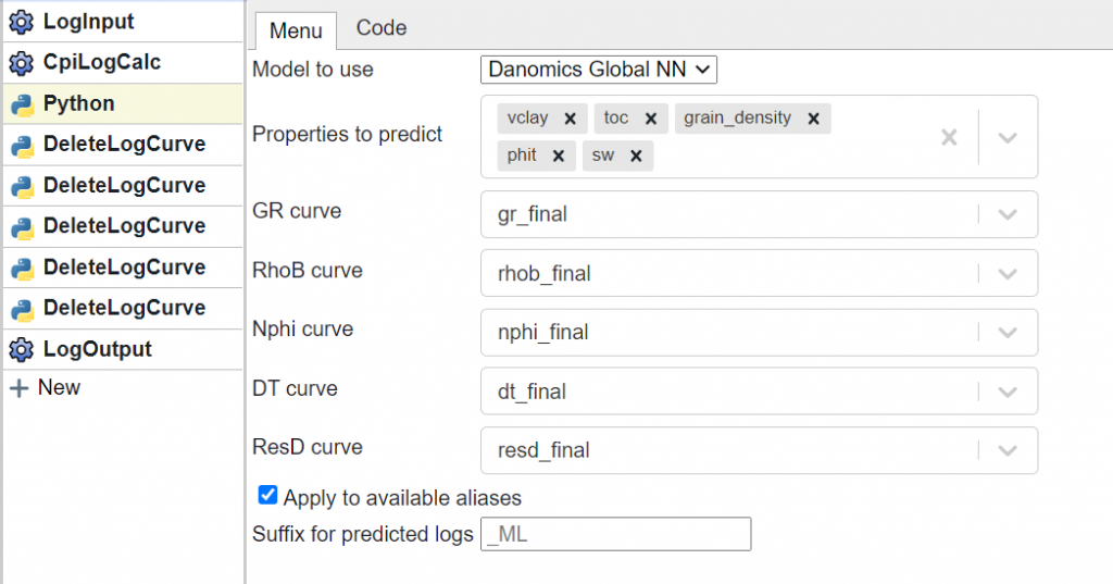
- PetrolML: Choose what properties to predict and what curves to use for prediction. There is also an option for which model to use. At present there is only one available model, but more models may be made available in the future.
- DeleteLogCurve: The CpiLogCalc block added the “_Final” curves to the log database – as further work will be performed on the resulting database, these were removed.
- LogOutput: Provide a name for the resulting database.
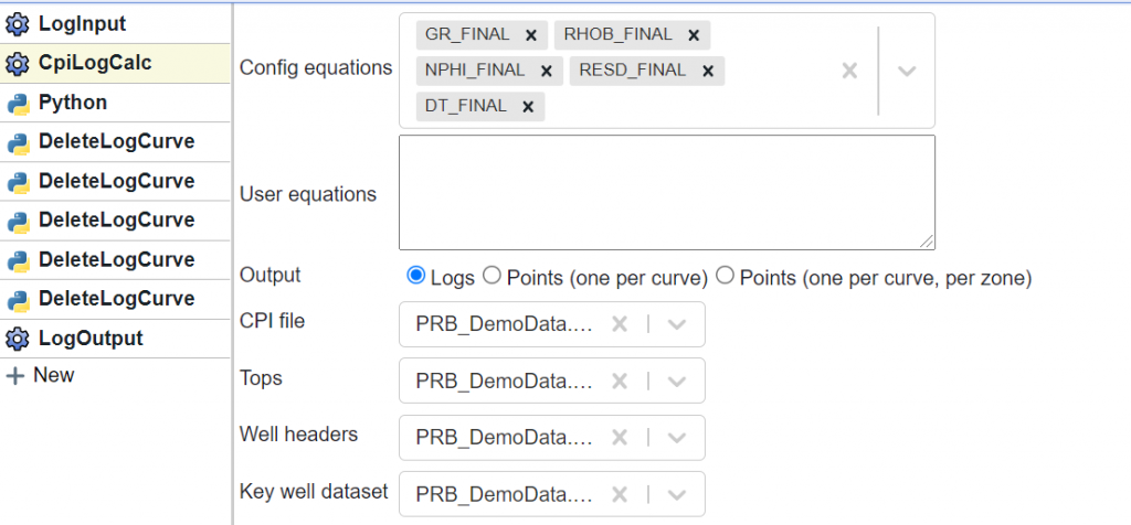
The CpiLogCalc block was used so that we could add the “_Final” curves to the Flow for use in the prediction. Note that you don’t need to provide a CPI file – if you do, it will use that CPI to apply things like normalization and washout repair. If you don’t select a CPI it will just access the config to composite, alias, and standardize curves.
Data Requirements
The petrophysical property prediction models try to apply a model that uses GR, RhoB, Nphi, DT, and ResD. If DT is not available it will attempt a prediction using a secondary model that does not use sonic as an input. Future work may include support for sparser curve datasets. Depth steps without GR, RhoB, Nphi, and ResD will not receive predictions Wells missing one of the required curves will also not receive a prediction.
Tips and Tricks
- Use the CpiLogCalc to access the “_Final” curves.
- Work a preliminary CPI through the Badhole ID & Repair module to ensure that you are not making predictions with data from washout intervals
- Each of the predicted properties uses its own individual models – evaluate each of the properties against a manual analysis to determine its usefulness.
- QC the results using maps and cross-sections
- Water saturation is the least reliable of the models – this is due to the multitude of factors that influence resistivity response. Consider performing a more rigorous QC of results including Sw.
Remember that if you need help that you can always reach us at support@danomics.com.