In Danomics Petrophysics users are guided through a workflow that walks them through a number of modules. These modules are located via a dropdown menu at the top center of the window. The modules are listed in the order in which a user should ideally proceed through a project. However, this order is not strictly enforced and the user can start at any module and can seamlessly move both forward and back through the modules. This help article will focus on the Cased Hole Interpretation module.
Cased Hole Interpretations
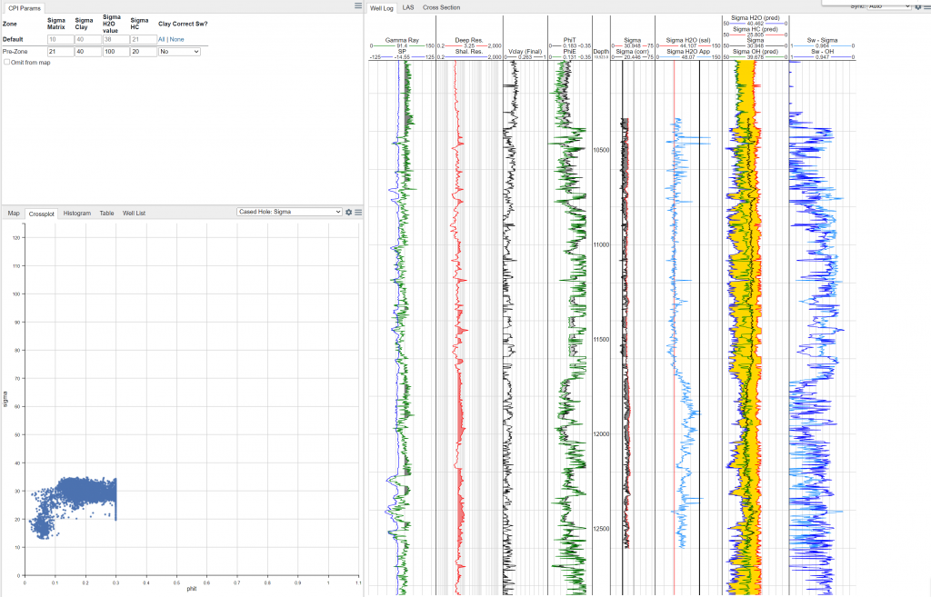
The cased hole interpretation module is designed to aid intepretations when there is a limited open hole suite or when a cased hole sigma log has been acquired and there is a desire to compare initial open hole water saturation calculations to subsequent saturations that may have been affected by water flooding or production. To access the module selected “Cased Hole Interpretation” from the module selection dropdown menu.
At present the module uses the sigma log to derive a cased hole saturation, while using the porosity and clay volumes calculated from the open hole logs. The user must enter parameters for the sigma values of the matrix, clay, water, and hydrocarbons and then select if a clay correction should be applied to the sigma curve before calculating the saturation.
Parameter Selection
Setting the parameters for sigma is crucial to calculating the Sw from the sigma log, which is essentially done via the distance between the end member points between the matrix-water and matrix-hydrocarbon points. This means at low porosity values (< 20%) and in fresh to brackish water systems (< 20k ppm) the method can be very unstable and will often bounce between very high and very low Sw values. However, in higher porosity and higher salinity systems the results can be quite robust.
Sigma Matrix should be set near the low end of the distribution of the sigma curve and can be done via the slider bar in the Sigma track (first track right of the depth track). It can also be useful to evaluate this in a crossplot of phit vs. sigma, where the sigma matrix value would be set at a value where phit equals 0.
Sigma Water is a function of the salinity. Values range from 22 for a freshwater system to 120 for a salt-saturated system (the correlation is linear). A sigma water apparent curve is calculated to help set the sigma water parameter in the case where the salinity is not known.
Sigma HC can vary from ~10 for a gas a reservoir P/T up to 21 for an oil at reservoir P/T.
To help in the QC process a track showing the measured sigma, sigma HC (predicted), sigma water (predicted) and sigma openhole (predicted) is given. If the measured sigma falls outside of the shaded range between the sigma water and sigma hydrocarbon predictions the input parameters may need to be revisited.
The results track shows the Sw from sigma in light blue and Sw from open hole in dark blue. If both were measured before any production or injection into the reservoir one would expect them to overlie one another if the model was properly calibrated and the system was amenable to Sw determinations from the sigma log (e.g., higher salinity and higher porosity).
Key Outputs
The primary output at this time is the water saturation from sigma, denoted as “sigma_sw”.