This article reviews how to modify interpretations well-by-well in the DCA tool. Once you have created a project, as outlined in this article, you should have a project that is fully populated with the default interpretation for every well already performed. However, you should set the global constraints on the analysis and perform updates on a well-by-well basis as needed.
Setting Global Contraints
As shown in the screenshot below, in the control panel on the right, there is a section called “Decline Curve Analysis”. Check the box “Constrained” to set global constraints on your project.
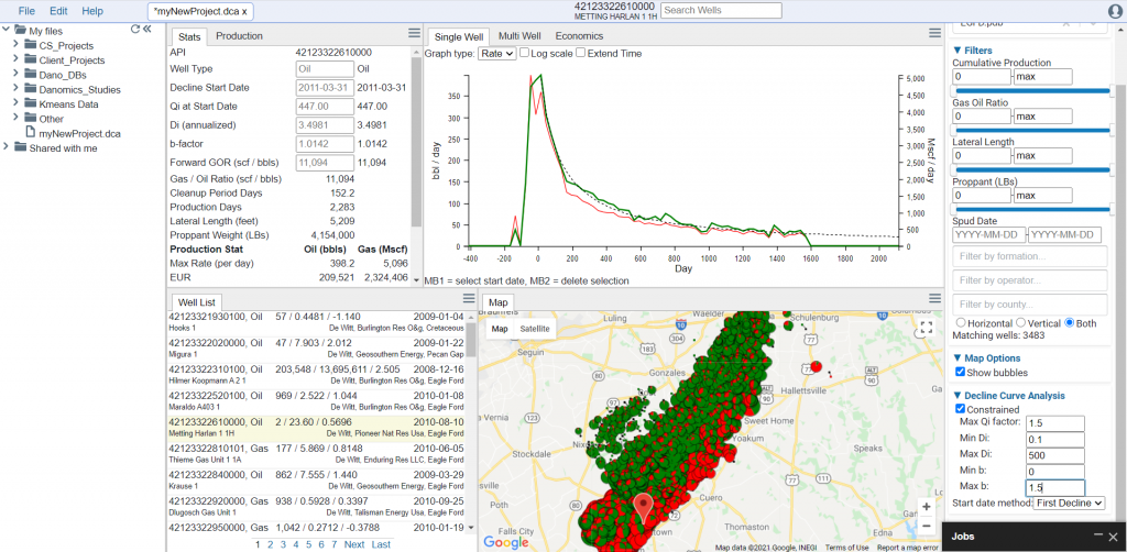
There are five value entry boxes Max Qi, Min Di, Max Di, Min b-factor, and Max b-factor. These correspond to the Qi, Di, and b-factor variables in Arp’s equation:
Q = Qi * (1+b*Di*t)^(-1/b)The Max Qi parameter establishes how high the theoretical Qi value is allowed to go relative to the maximum reported production for any given time period. The value should be lower for daily production and higher for monthly or annual production. The value should never be set less than 1.
The Di is a unitless decline factor. By keeping this unitless it is time-independent, so you can change from daily to monthly to annually reported data without worrying about modifying it. It is recommended to have a range of 0 < Di <=500. Therefore, we set Min Di at 0.01 and Max Di at 500 as a starting point.
The b-factor should be in the range of 0 <= b <= 2. The upper and lower bounds are constrained by physics-based solutions. In most cases, however, 0 <= b <= 1.5. A good way to determine this is to set it at a value of 2, export your results, and then evaluate the range of b-factors. Usually a trend will emerge on wells with higher confidence interpretations (longer production histories) that will show b-factors are typically well below 2.
Start Date Method
One of the trickiest parts of the automated interpretation is determining how to set the start date in the decline. This is complicated by clean-up periods during flowback after completion, production constraints that create an artificially low first few months of production, and late-in-life recompletions if your focus is on forward-looking forecasts only.
The “Best Fit” option attempts to perform a curve fit at every possible increment and selects the best one, with an increasing penalty with time. This means that it tries to start earlier in well life, but if the fit is significantly better in late life, the decline may start later in the well life. This makes it ideal for evaluating forward looking production.
The “First Decline” option starts at the first observed decline. This is often ideal for constrained production where monthly rates are capped for several reporting periods.
“Max” means that the decline will start at the reporting period with the maximum reported rate. This is typically ideal for unconventional resource plays and for evaluating overall well performance. It is recommended to use this as a starting point.
Once these options have been set the analysis on every well will be updated to reflect these changes.
Single-well Updates
Although all interpretations are performed automatically you have full control to update the DCA results for each well.
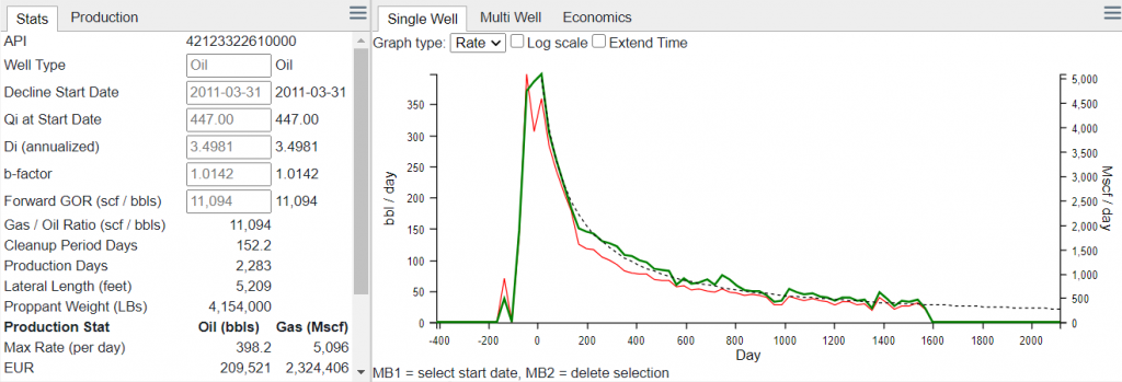
In the “Stats” tab there are options for well type, start date, Qi, Di, b-factor, and Forward looking GOR.
For Well Type the options can be set to either “Oil” or “Gas”. This is determined based on GOR, but can be manually overridden. It should reflect your primary fluid.
For Decline Start Date you can set this by either left-clicking on the production graph or by entering a date in yyyy-mm-dd format.
Qi, Di, and b-factor can be overridden by typing a value into the box. Note that when you change one value the other two will automatically change to maintain the best possible fit. In most cases you will want to set the b-factor first, and then the Di if needed and finally the Qi.
Filtering the Data
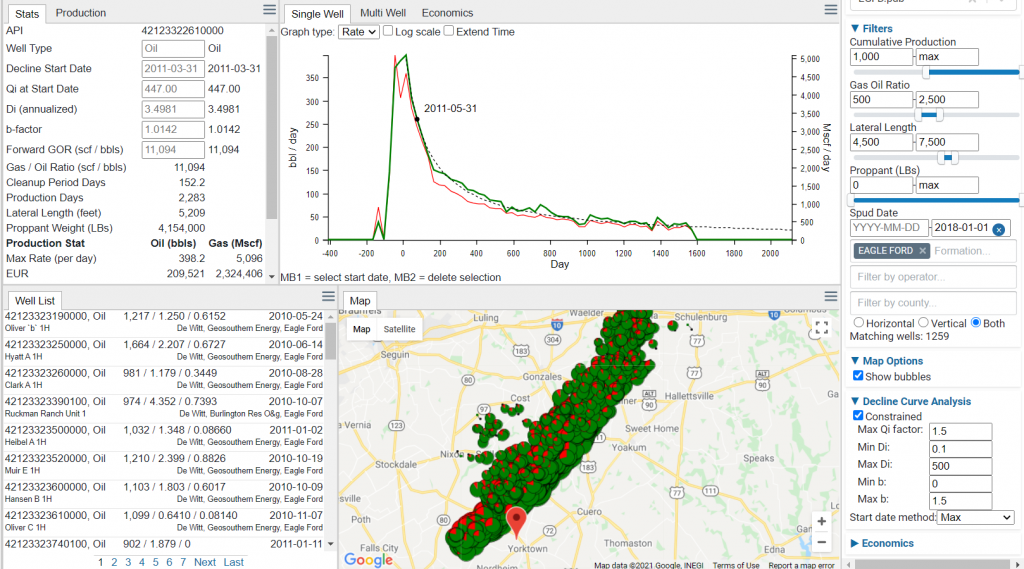
It is likely that you will want to filter your data to the wells that are relevant to your analysis. To do this you can set filters in the control panel on the right hand side.
It is typically useful to at least set a minimum value for the cumulative production (in BOEs) as this will filter out wells that do not have significant histories. The Gas-oil Ratio filter can be set to the desired range, as can lateral length and proppant volume. For Spud Date it is often important to set the date such that one will have at least 6-12 months of production history as this much is often needed to obtain a good fit for the DCA.
Filters can also be set for Formation, Operator, and County, on an as-needed basis.
Tips and Tricks
- During the QC process, you can click on a well in the well list, and then use the down arrow to advance to the next well. This will allow you to rapidly evaluate wells.
- Experiment with the start date method to see how it affects results. Max and Best Fit are typically the best options.
- Remember what is important to your analysis – do you want to evaluate only remaining reserves? If so, the Best Fit option is likely the best option. If you want to evaluate overall new well performance, the Max option is likely better.