Geology. Petrophysics. 100X Faster.
Scale to 1000s of wells with the only subsurface platform built for 2030.


Trusted by 100s of geologists and petrophysicists at top oil & gas companies
Maximize the value of the subsurface
Build
Structural & stratigraphic framework

Calculate
the key reservoir properties & volumetrics

Generate
3D reservoir property models & visualizations

Here’s your new subsurface workflow
Import the data
Choose your target
Import well headers, logs, tops, core data, shapefiles, and more in widely popular formats.
Maps and cross-sections
Build the framework
Generate structure and isopach maps with special built tools that honor geological principals and rapidly pick tops with assisted tops correlation.
Calculate key reservoir properties
Scale to 1000s of wells
Rapidly scale your interpretation to 1000s of wells and customize interpretations using our spatial interpolation tools.
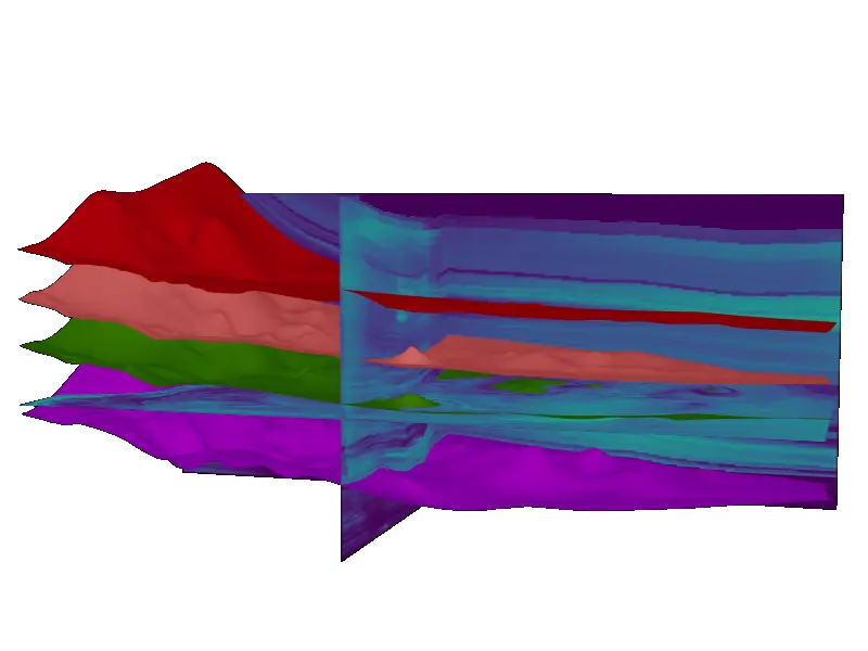
Generate 3D Property Models
Gain insights through 3D models
Rapidly move from logs to maps to 3D models and extract properties into horizontal producers for deeper insights into production drivers.